Building Latent Class Trees, With an Application to a Study of Social Capital

Standard LC Analysis

Let y_ij denote the response of individual i on the jth of J categorical response variables. The complete vector of responses of individual i is denoted by y_i. In a latent class analysis, one defines a model for the probability of observing y_i; that is, for P(y_i). Denoting the discrete latent class variable by X, a particular latent class by k, and the number of latent classes by K, the following model is specified for P(y_i):

Here, P(X = k) represents the (unconditional) probability of belonging to class k and P(y_ij|X = k) represents the probability of giving the response concerned conditional on belonging to class k. The product over the class-specific response probabilities shows the key model assumption of local independence.

Latent class models are typically estimated by maximum likelihood, which involves finding the values of the unknown parameters maximizing the following log-likelihood function:

Here, θ denotes the vector of unknown parameters and N the total sample size, and P(y_i) takes the form defined in Equation 1. Maximization is typically done by means of the expectation-maximization (EM) algorithm.

Building a LCT

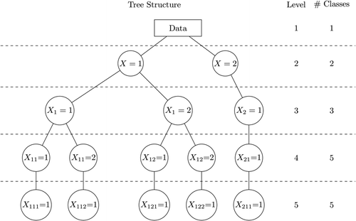
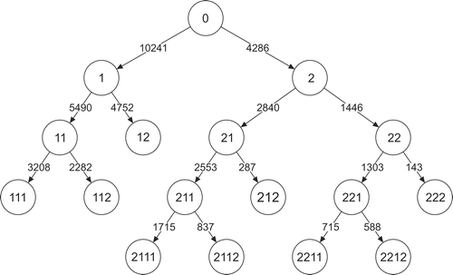
The building of a LCT involves the estimation and comparison of 1- and 2-class models only. If a 2-class solution is preferred over a 1-class solution (say, based on the BIC), the sample is split into two subsamples and 1- and 2-class models will subsequently be estimated for both newly formed samples. This top-down approach continues until only 1-class models are preferred, yielding the final hierarchically ordered LCT. An example of such a LCT is depicted in Figure 1. The top level contains the root node which consists of the complete sample. After estimating 1- and 2-class models with the complete sample, it is decided that the 2-class model is preferred, which implies that the sample is split into two subsamples (class X = 1 and class X = 2), which form level 2 of the tree. Subsequently, class 1 is split further while class 2 is not, yielding classes X₁ = 1, X₁ = 2, and X₂ = 1 at level 2. In our example, after level 4 there are no splits anymore and hence the final solution can be seen at both levels 4 and 5. Though level 5 is redundant, this is only visible after the procedure has been finished; that is, after only 1-class models are preferred.

More formally, the 2-class LC model defined at a particular parent node can be formulated as follows:

A key issue for the implementation of the divisive LC algorithm is how to perform the split at the parent node when a 2-class model is preferred. As proposed by Van der Palm et al. (2016), we use a proportional split based on the posterior class membership probabilities, conditional on the parent node, for the two child nodes, denoted by k = 1, 2. These are obtained as follows:

Estimation of the LC model at the parent node X_parent involves maximizing the following weighted log-likelihood function:

In other words, a weight at a particular child node equals the weight at its parent node times the posterior probability of belonging to the respective child node, conditional on belonging to the parent node. As an example, the weights used for investigating a possible split of class X₁ are constructed as follows:

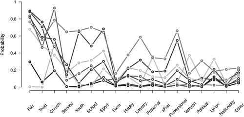
Construction of a LCT can thus be performed using standard software for LC analysis, namely by running 1- and 2-class models multiple times with the appropriate weights. We developed an R routine in which this process is fully automated.¹ It calls the Latent GOLD program (Vermunt & Magidson, 2013) in batch mode to estimate the 1- and 2-class models, evaluates whether a split should be made, and keeps track of the weights when a split is accepted. In addition, it creates several types of graphical displays which facilitate the interpretation of the LCT. A very useful and novel graphical display is a tree depicting the class-specific response probabilities P(y_ij|X_child = k, X_parent) for the newly formed child classes using profile plots (e.g., see Figure 2). In this tree, the name of a child class equals the name of the parent class plus an additional digit, a 1 or a 2. The structure of the tree will in principle be affected by label switching resulting from the fact the order of the newly formed classes depends on the random starting values. To prevent this when building the LCT, our algorithm locates the larger class at the left branch with number 1 and the smaller class at the right branch with number 2.

Statistics for Building and Evaluating a LCT

In a standard LC analysis, one will typically estimate the model for a range of number of classes K, say from 1 to 10, and select the model that performs best according to the chosen fit index. The most popular measures are information criteria such as BIC, AIC, and AIC3, which aim at balancing model fit and parsimony (Andrews & Currim, 2003; Nylund, Asparouhov, & Muthén, 2007). Denoting the number of parameters by P, these measures are defined as follows:

These indices penalize a larger number of parameters differently. AIC3 will favor a more parsimonious model, that is, with a smaller or equal number of classes, than AIC. BIC typically favors an even more parsimonious model, because log(N) is usually larger than 3.

As in a standard LC model, we need to decide, which model should be preferred, with the difference that here we only have the choice between 1- and 2-class models. This decision has to be made at each node in the tree. In the empirical example presented in the next section, we will base this decision on the BIC, which means that we emphasize the parsimony of a model. However, in the evaluation of the tree, we will also investigate which splits rejected by BIC would be accepted by AIC3. In the computation of the BIC, we use the total sample size, and thus not the sample size at the node concerned. Note that classes are split as long as the difference between the BIC of the estimated 1- and 2-class models, ΔBIC = BIC(1) − BIC(2), is larger than 0. The size of ΔBIC can be compared across splits, where larger ΔBIC values indicate that a split is more important; that is, it yields a larger increase of the log-likelihood and thus a larger improvement of fit.

Another possible way to assess the importance of a split is by looking at the reduction of a goodness-of-fit measure such as the Pearson chi-square. Because overall goodness-of-fit measures are not very useful when the number of response variables is large, we will use a goodness-of-fit measure based on the fit in two-way tables. The fit in a two-way table can be quantified using the bivariate residual (BVR), which is a Pearson chi-square statistic divided by the number of degrees of freedom (Oberski, van Kollenburg, & Vermunt, 2013). A large BVR value indicates that the association between that pair of variables is not picked up well by the LC model or, alternatively, that the local independence assumption does not hold for the pair concerned. By summing the BVR values across all pairs of variables, we obtain what Van Kollenburg, Mulder, and Vermunt (2015) refer to as the total BVR (TBVR):

A split is more important if it yields a larger reduction of the TBVR between the 1- and 2-class solution. In other words, we look at: ΔTBVR = TBVR(1) − TBVR(2).

While ΔBIC and ΔTBVR can be used to determine the importance of the splits in terms of model fit, it may also be relevant to evaluate the quality of splits in terms of their certainty or, equivalently, in terms of the amount of separation between the child classes. This is especially relevant if one would like to assign individuals to the classes resulting from a LCT. Note that the assignment of individuals to the two child classes is more certain when the larger of the posterior probabilities P(X_child = k|y_i; X_parent) is closer to 1. A measure to express this is the entropy; that is,

Typically Entropy (X_child|y) is rescaled to lie between 0 and 1 by expressing it in terms of the reduction compared to Entropy (X_child), which is the entropy computed using the unconditional class membership probabilities P(X_child = k|X_parent). This so-called R²_Entropy is obtained as follows:

Building the LCT

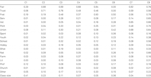
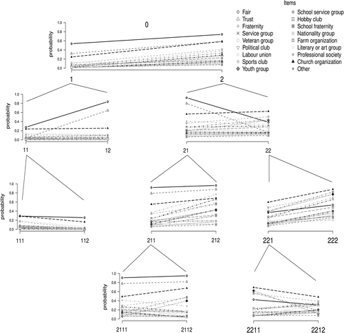
The proposed LCT methodology is illustrated by a reanalysis of a large data set which was previously analyzed using a standard LC model. Owen and Videras (2009) used the information from 14.527 respondents of the 1975, 1978, 1980, 1983, 1984, 1986, 1987 through 1991, 1993, and 1994 samples of the General Social Survey to construct a typology of social capital that accounts for the different incentives that networks provide. The data set contains 16 dichotomous variables indicating whether respondents participate in specific types of voluntary organizations (the organizations are listed in the legend of Figure 2) and two variables indicating whether respondents agree with the statements that other people are fair and other people can be trusted. Owen and Videras explain the inclusion of the latter two variables by stating that social capital is a multidimensional concept which includes both trust and fairness as well as multiple aspects of civic engagement. Using the BIC, Owen and Videras selected a model with eight classes, while allowing for one local dependency, namely between the items fraternity and school fraternity.

Figure 2 depicts the results obtained when applying our LCT approach using the BIC as the splitting criterion. A figure of a tree containing information on the sample sizes and the different nodes is provided in Appendix A. As can be seen, at the first two levels of the tree, all classes are repetitively split. However, at the third level only three out of four classes are split, as a division of class 12 is not supported by the BIC. Subsequently, the number of splits decreases to two at the fourth level, while at the fifth level there are no more splits, indicating the end of the divisive procedure.

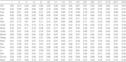
For the interpretation of the LCT, we can use the profile plots, which show which variables are most important for the split concerned (exact probabilities can be found in Appendix B). From the upper panel of Figure 2, which depicts class-specific response probabilities for classes 1 and 2, it can easily be seen that all probabilities are higher for class 2 than for class 1, which is confirmed by Wald tests (W ≥ 7.43, p < .05). So basically the first split divides the sample based on general social capital, where class 1 contains respondents with low social capital and class 2 respondents with high social capital. This is supported by the total group participation of each class (TGP, the sum of all probabilities except fair and trust), which equals 0.88 for class 1 and 3.83 for class 2.

The second row of Figure 2 shows the splitting of both classes 1 and 2 is mainly due to the variables fair and trust. Apparently the low and high social capital groups can both be split based on how respondents view other people regarding fairness and trustworthiness. This categorization will be called optimists versus pessimists. The difference in TGP is relatively small for these two splits, being 0.09 between class 11 and 12 and 0.83 between class 21 and 22. Up to here, there are four classes: pessimists with low social capital (11), optimists with low social capital (12), optimists with high social capital (21), and pessimists with high social capital (22).

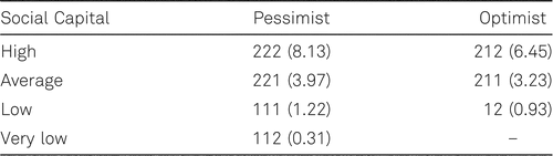
Looking at the next level, one can see that class 12 is not split further. The third row of Figure 2 shows similar patterns for all three splits at this level: all probabilities are lower in one class than in the other. Therefore these splits can be interpreted as capturing more refined quantitative differences in social capital. This results in seven classes, ranging from high to very low social capital, as can be seen from the TGP values reported in Table 1.

Table 1 Interpretation of classes at level 3 with TGP in parentheses

Social Capital	Pessimist	Optimist
High	222 (8.13)	212 (6.45)
Average	221 (3.97)	211 (3.23)
Low	111 (1.22)	12 (0.93)
Very low	112 (0.31)	–

Table 1 Interpretation of classes at level 3 with TGP in parentheses

View as image HTML

At the fourth level, both the optimists and pessimists classes with average social capital (211 and 221) are split. Contrary to the previous splits, here we can see qualitative differences in terms of the type of organization in which one participates. For instance, in classes 2112 and 2211, respondents have higher probabilities of being a member of a sports or a youth group, while in the corresponding classes 2111 and 2212, respondents have a higher probability of being a member of a professional organization. The TGPs of the newly formed classes are similar, ranging between 3.17 and 4.06, while fair and trust are high at the optimistic branch and low at the pessimistic branch of the tree. At level five no further splits occur.

At the lowest level, the constructed LCT has nine classes, one more than obtained with a standard LC analysis. It turns out that the classes identified with the two alternative approaches are rather similar. The parameters from the standard eight-class model appear in the profile plot depicted in Figure 3 and in Appendix C. For instance, the conditional probabilities of LC-class 1 are very similar to those of LCT-classes 111 and 112. Moreover, LC-class 1 is even more similar to the higher-order LCT-class 11, which suggests that the distinction between LCT-classes 111 and 112 is probably not made in the standard LC analysis. The three largest classes of the original analysis are very similar to at least one LCT-class (LC 1 to TLC 11, LC 2 to LCT 12, and LC 3 to LCT 2111), while three out of the five smaller original classes can also be directly related to a LCT-class (LC 6 to LCT 221, LC 7 to LCT 2112, and LC 8 to LCT 222). LC-classes 4 and 5 (containing 7% and 5% of the respondents) are not clearly related to a LCT-class.

Evaluating the Splits of the LCT

Now let us look in more detail at the model fit and classification statistics associated with the accepted and rejected splits. Table 2 reports the values of ΔBIC, ΔAIC3, ΔTBVR, and R²_Entropy, as well as the class proportions, for the considered splits, where the classes split based on the ΔBIC appear in the top rows and the others in the bottom rows. Looking at the ΔAIC3, we can see that this criterion would have allowed (at least) five additional splits. The ΔTBVR values show the fit always improves, but the improvements are larger for the accepted than for the rejected splits. The R²_Entropy indicating the quality of a split in terms of classification performance, shows a rather different pattern: it takes on both higher and lower values among accepted and non-accepted splits.

Table 2 Information criteria per split, with split classes in the top and not split classes in the bottom rows

	BIC	AIC3	TBVR	R2Entropy	P(X = k)
0	9,205.4	9,330.5	23,597.7	0.648	1.000
1	1,346.2	1,471.3	1,495.0	0.489	0.705
2	691.0	816.1	1,071.4	0.516	0.295
11	30.8	155.9	279.1	0.261	0.378
21	117.7	242.8	275.6	0.512	0.195
22	94.9	220.0	285.2	0.610	0.100
211	92.9	218.0	338.2	0.353	0.176
221	58.6	183.7	313.9	0.433	0.090
12	−37.7	87.4	179.4	0.222	0.327
111	−84.3	40.8	100.5	0.295	0.221
112	−167.3	−42.2	16.4	0.174	0.157
212	−125.5	−0.4	72.3	0.473	0.020
222	−119.0	6.1	64.6	0.815	0.010
2111	−2.7	122.4	206.0	0.353	0.118
2112	−126.7	−1.6	63.7	0.288	0.058
2211	−136.4	−11.4	54.8	0.257	0.049
2212	−99.1	26.0	100.6	0.383	0.041

Table 2 Information criteria per split, with split classes in the top and not split classes in the bottom rows

View as image HTML

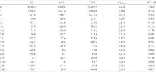
Based on the information provided in Table 2, one could opt not to split class 11. Compared to other accepted splits, splitting this class contributes much less in terms of improvement of fit, while also the classification performance associated with this split is rather bad. Note also that this is one of the largest classes and therefore the statistical power to retrieve subclasses with small differences is relatively high. The decision on retaining this split depends on whether the encountered more detailed distinction within this low social capital and pessimistic class is of substantive interest. However, what is clear is that if a good classification performance is required, this split seems to be less appropriate.

Conversely, one might want to include the split of class 2111. Though this split was rejected by the ΔBIC stop criterion, this is based on a rather small negative value, while the values for the ΔAIC3 and ΔTBVR are relatively high. However, the R²_Entropy indicates a low quality of this split. Hence, the information on the fit improvement might be misleading, due to this class being the largest class at the lowest level of the tree.

The opposite is true for the split of class 222. Though this class is quite small and the fit statistics of this split indicate not much improvement, the R²_Entropy indicates that classes 2221 and 2222 would be very well separated. Of course, once again the research question at hand is crucial for the decision to add a class to the tree. For exploration the split of class 2111 can be relevant, while for classification the split of class 222 might be more appropriate.

References

(2003). A comparison of segment retention criteria for finite mixture logit models. Journal of Marketing Research, 40, 235–243. doi: 10.1509/jmkr.40.2.235.19225
(1995). Latent class models. Handbook of statistical modeling for the social and behavioral sciences. New York, NY: Springer, 311–359.
(2002). Cluster merging and splitting in hierarchical clustering algorithms.Proceedings of the 2002 IEEE International Conference on Data Mining (ICDM’02), Japan Retrieved from https://pdfs.semanticscholar.org/6daf/9d571510b087638afdf744f34deb391529c5.pdf. doi: 10.1109/ICDM.2002.1183896
(2011).
Hierarchical clustering . In W. A. ShewhartS. S. WilksEds., Cluster analysis (5th ed., pp. 71–110). Chichester, UK: Wiley.(2009). The elements of statistical learning, Data mining, Inference and Prediction. (Vol. 2), New York, NY: Springer.
(1974). Exploratory latent structure analysis using both identifiable and unidentifiable models. Biometrika, 61, 215–231.
(1990). Categorical longitudinal data: Log-linear panel, trend, and cohort analysis. Newbury Park, CA: Sage.
(2010). Methods for merging Gaussian mixture components. Advances in data analysis and classification, 4, 3–34.
(2013). How to find an appropriate clustering for mixed-type variables with application to socio-economic stratification. Journal of the Royal Statistical Society: Series C (Applied Statistics), 62, 309–369.
(1968). Latent structure analysis. Boston, MA: Houghton Mifflin.
(1997). Split selection methods for classification trees. Statistica Sinica, 7, 815–840.
(1987). Latent class analysis (Quantitative Applications in the Social Sciences, No. 64). Thousand Oaks, CA: Sage.
(2007). Deciding on the number of classes in latent class analysis and growth mixture modeling: A Monte Carlo simulation study. Structural Equation Modeling, 14, 535–569.
(2013). A Monte Carlo evaluation of three methods to detect local dependence in binary data latent class models. Advances in Data Analysis and Classification, 7, 267–279.
(2009). Reconsidering social capital: A latent class approach. Empirical Economics, 37, 555–582.
(1978). Estimating the dimension of a model. The Annals of Statistics, 6, 461–464.
(2016). Divisive latent class modeling as a density estimation method for categorical data. Journal of Classification, 33, 52–72. doi: 10.1007/s00357-016-9195-5
(2015). Assessing model fit in latent class analysis when asymptotics do not hold. Methodology, 11, 65–79.
(2002).
Latent class cluster analysis . In J. HagenaarsA. McCutcheonEds., Applied latent class analysis (pp. 89–106). Cambridge, UK: Cambridge University Press.(2013). Technical guide for Latent GOLD 5.0: Basic, advanced, and syntax. Retrieved from https://www.statisticalinnovations.com/wp-content/uploads/LGtecnical.pdf
(2004). Hierarchical latent class models for cluster analysis. Journal of Machine Learning Research, 5, 697–723.
(2005). Hierarchical clustering algorithms for document datasets. Data Mining and Knowledge Discovery, 10, 141–168.
Appendix A
A Class Sizes of LCT