Factor Score Path Analysis
An Alternative for SEM?
Abstract
Abstract. Theoretical researchers consider Structural Equation Modeling (SEM) to be the preferred method to study the relationships among latent variables. However, SEM has the disadvantage of requiring a large sample size, especially if the model is complex. Furthermore, since SEM estimates all parameters simultaneously, one misspecification in the model may influence the whole model. For these reasons, applied researchers often use a two-step Factor Score Regression (FSR) approach. In the first step, factor scores are calculated for the latent variables, which are used to perform a linear regression in the second step. However, this method results in incorrect regression coefficients. Croon (2002) developed a method that corrects for this bias. We combine this method of Croon (2002) with path analysis, resulting in Factor Score Path Analysis. This method results in correct path coefficients and has some advantages over SEM: it requires smaller sample sizes, can handle more complex models and the method is less sensitive to misspecifications, because of its stepwise nature. In conclusion, this method can be a suitable alternative for SEM, when one is dealing with a complex model and small sample sizes.
Theoretical researchers consider Structural Equation Modeling (SEM) to be the preferred method to study the relationships among latent variables. SEM is a full information method that estimates all parameters simultaneously and results in unbiased estimates. In theory, SEM works perfectly. In practice, the method can have some drawbacks. A first issue is that SEM requires a large sample size, especially if the model is complex (Schumacker & Lomax, 1996; Valluzzi, Larson, & Miller, 2003). If the sample size is too small, the model may simply not converge and if it converges, the parameter estimations may be biased (Gagne & Hancock, 2006). A second issue originates from the simultaneous estimation of all parameters in the model. As a result, a misspecification in one part of the model may influence other parts of the model. For example, misspecifications in the structural model may bias the estimates in the measurement model.
For these reasons, limited information methods have been developed that attempt to overcome the drawbacks of SEM. For example, to overcome the misspecification issue, Bollen (1996) proposed the instrumental variables approach. This approach reduces the complexity of the model by using one indicator per latent variable as a scaling variable. Then, the structural equations are reformulated to use this scaling variable instead of the latent variables, resulting in equations with only observed variables. These equations are finally solved using a two-stage least squares estimator. To overcome the sample size issue, applied researchers have often used the two-step Factor Score Regression (FSR) approach (Lu, Kwan, Thomas, & Cedzynski, 2011). In this approach, the first step is to perform a factor analysis and to calculate factor scores for each latent variable. These factor scores are estimates for the true latent variable scores. There are several predictors that can be used to compute the factor scores, but the two most commonly used predictors in the continuous case are the regression predictor (Thomson, 1934; Thurstone, 1935) and the Bartlett predictor (Bartlett, 1937; Thomson, 1938). In a second step, the factor scores are used in a linear regression, as if they were the true latent variable scores. By using FSR, the number of models that do not converge, is reduced. However, while this method has less problems with convergence, the use of factor scores results in biased estimates of the regression parameters, even when the sample size is large.
Several methods were developed that account for this bias. Skrondal and Laake (2001) developed a FSR method that avoids the bias by using the regression predictor for the independent latent variables and the Bartlett predictor for the dependent latent variables. However, when there are correlations between the independent variables, this method can no longer be used. Croon (2002) developed a FSR method that corrects for the bias. This method is based on the premise that there is a difference between the variances and covariances of the factor scores and the variances and covariances of the true latent variable scores. Croon (2002) uses an estimation of the variances and covariances of the true latent variable scores, instead of the factor scores, to estimate the regression parameters. A similar approach has been discussed in Hoshino and Bentler (2013). The method of Hoshino and Bentler (2013) only uses the Bartlett predictor and relies on weighted least squares (WLS) estimation, while the method of Croon (2002) can be used with any predictor and any estimator. In his paper, Croon (2002) only discussed the method from a population point of view and did not study how the method performs in finite samples. This was done by Lu et al. (2011) and by Devlieger, Mayer, and Rosseel (2016). Both concluded that the method of Croon (2002) results in unbiased parameter estimates when finite samples are used. Devlieger et al. (2016) also showed that the method has a comparable efficiency, mean square error, power, and type I-error rate as SEM, when the sample size is large. However, despite these encouraging results, many questions about this method still remain. For example, how does the method compare to SEM with regard to its main drawbacks, namely settings with small sample sizes and misspecifications? And can the method be extended to be used with path analysis? The goal of this paper is to answer these questions.
The rest of the paper is organized as follows. First, we outline the method of Croon, including a step-by-step description of how to perform the method using path analysis. Next, two simulation studies will be presented. In these studies, the performance of the method of Croon will be compared to the performance of SEM. The first study uses a correctly specified and two incorrectly specified models. The goal of this study is to evaluate the finite sample performance of the method of Croon using path analysis and to compare the robustness of SEM and the method of Croon to misspecifications in the model. The second study uses a more complex, but correctly specified model, and smaller sample sizes. The aim of this study is to compare the performance of both methods when the sample size is small.
The Method of Croon
The Method of Croon Using Regression Analysis
Croon (2002) developed the method to be used in general latent variable models, meaning all models that include latent variables. He uses univariate and multivariate regression settings with several latent variables to explain the method. The simple regression model in Figure 1 is an example of this setting.
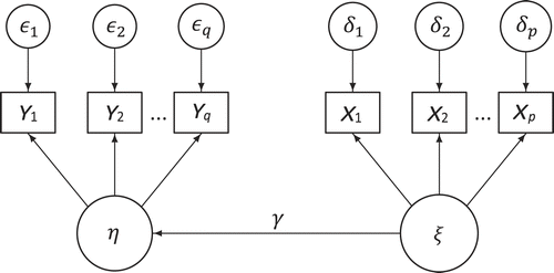
The first step of the method is to use the measurement models to perform a factor analysis for each latent variable separately and to calculate their respective factor scores, Fξ and Fη. As we mentioned before, there are several predictors that can be used to compute these factor scores, such as the regression predictor and the Bartlett predictor. In this paper, the regression predictor will be used.
The second step of FSR methods is to perform a linear regression between the factor scores, resulting in a regression coefficient. In a simple linear regression, the true regression coefficient is defined as the true covariance between the dependent and the independent variable, multiplied by the inverse of the true variance of the independent variable:
When performing the linear regression with factor scores, the regression coefficient is defined as the covariance between the factor scores of the dependent and the independent variable, multiplied by the inverse of the variance of the factor scores of the independent variable:
Croon (2002) has shown that γ and β are not equal in all conditions, since there is a difference between the variances and covariances of the factor scores (ΣFS) and the variances and covariances of the true latent variable scores (Ση). For this reason, Croon (2002) uses estimates of the variances and covariances of the true latent variable scores ( ) instead of ΣFS. The variances and covariances of the true latent variable scores can be estimated as follows:


For more details on how these formulas were derived, the interested reader is referred to (Croon, 2002) and (Devlieger et al., 2016).
The Method of Croon Using Path Analysis
When the model includes a mediational relationship, it is not possible to perform one single linear regression. For recursive models such as the full mediation model in Figure 2A or the partial mediation model in Figure 2B, it is possible to perform a series of linear regression analyses, one per endogenous variable. The full mediation model could also be analyzed using the method of Skrondal and Laake (2001), but note that the method would fail for the partial mediation model, due to the correlation between η1 and η2.
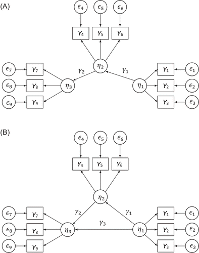
However, this multiple regression strategy can only be used for recursive path models. For non-recursive path models (having reciprocal effects, loops, or bow-pattern disturbance correlations), a simultaneous estimation method like maximum likelihood (ML) is required (Kline, 2015). Therefore, we apply the principle of the method of Croon to path analysis. When using path analysis, the method can be summarized as follows:
- 1.Perform factor analysis for all latent variables separately and calculate their respective factor scores.
- 2.Calculate the variance-covariance matrix of the factor scores (ΣFS).
- 3.Estimate the true variances and covariances for all elements in this variance-covariance matrix (
 ).
). - 4.Perform a path analysis, using the estimated variances and covariances
 as the input covariance matrix for the model.
Combining the method of Croon and path analysis means non-recursive models can be analyzed using factor scores, without bias. An example, using a bow-pattern model, is given in Figure 3.
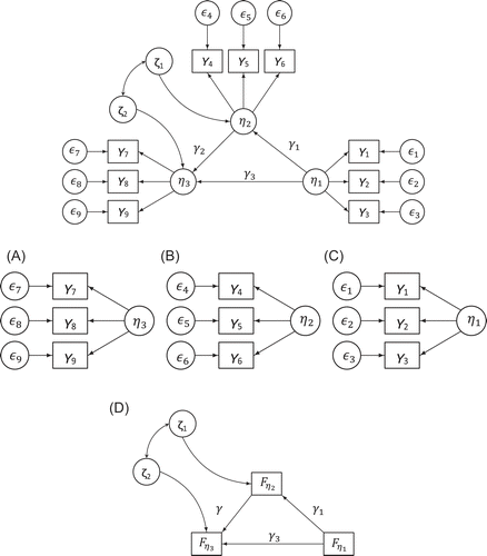
 ). (D) Perform a path analysis, using the estimated variances and covariances
  as the input covariance matrix for the model.
Simulation Studies
Simulation Study 1: Path Analysis and Misspecifications
Data Simulation
The data of the first study was simulated using the ground truth model depicted in Figure 4. The data was simulated in R (R Development Core Team, 2016). The true latent variable scores were generated first. The variances of the exogenous variables, ξ1, ξ2, and ξ3, were set at 100, while the residual variances of the endogenous variables η1 and η2 were both set at 400. The true latent scores of ξ1, ξ2, and ξ3 were generated first, followed by the regression residuals ζ1 and ζ2, all by drawing from a univariate normal distribution. Finally, using the structural equations η1 = γ1 ξ1 + γ2 ξ2 + ζ1 and η2 = γ3 ξ3 + γ4 ξ1 + γ5 η1 + ζ2, the true latent scores on η1 and η2 were generated. γ1, γ2, γ3, and γ4 were set at 1.5, while γ5 was set at a value of 0.51.
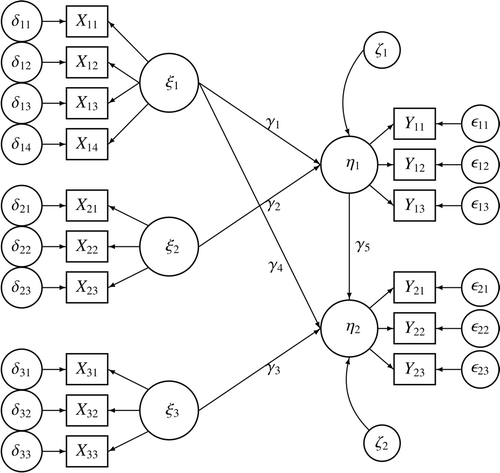
Then, data for each observed item response xlm and ylm was generated, with the “l” index referring to the latent variables and the “m” index referring to the items. The measurement models of the latent variables were ylm = λylm ηl + ϵlm and xlm = λxlm ξl + δlm. All factor loadings were set at 1. The residual variances were set at  and
and  , with CDyl and CDxl the coefficients of determination for the measurement models, respectively. All CDxl and CDyl are equal and will thus be referred to as CD. The coefficients of determination CD were varied between 0.3, 0.6, 0.7, and 0.9. The sample size was set at 500, 1,000, or 2,000. Together, this created 12 experimental conditions.
Analyses
For each of the 12 conditions, 1,000 datasets were generated and then analyzed with both the method of Croon and SEM, using a “maximum likelihood” estimator. For the SEM approach, lavaan (Rosseel, 2012) was used. For the Croon method, lavaan (Rosseel, 2012) was used to calculate the factor scores and our own written routines were used to compute the Croon corrections and the resulting regression coefficients of the structural part of the model. For both methods, three different models were fitted to the data. The first model was correctly specified, creating a condition where SEM works optimally (Model 1). The two other models were misspecified models, one misspecification in the structural model and one misspecification in the measurement model. For the measurement misspecification (Model 2), item X4 was set to measure ξ2 instead of ξ1. For the structural misspecification (Model 3), the regression parameter γ4 was fixed to 0. This means there is no longer a direct effect of ξ1 on η2, but there is still a mediated effect through η1. For each model, the five regression coefficients γi were obtained for both methods. Based on the 1,000 replications, two performance criteria were computed, namely the convergence rate and the bias of each regression coefficient.
Results
Convergence Rate
The convergence rate for all three models is depicted in Figure 5. When the model is correctly specified or when there is a structural misspecification, both the method of Croon and SEM had a convergence rate of 100% in every condition. When there is a measurement misspecification, the convergence rate drops for both methods, but more severely for SEM. The convergence rate ranges from 0.701 to 0.911 for the method of Croon, while it ranges from 0.386 to 0.827 for SEM.

In conclusion, the method of Croon does indeed converge more often than SEM, when there are measurement misspecifications in the model. It is important to know if the method not only converges, but also results in reliable parameter estimates. For this reason, we also study the bias.
Bias
When the model is correctly specified, both methods show almost no bias (Figure 6A). However, there is a difference between the two methods. SEM tends to slightly overestimate, while the method of Croon tends to underestimate the regression coefficient. The small bias that can be found, disappears with growing sample size and coefficient of determination.
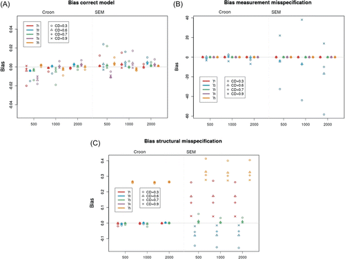
When looking at Figure 6B, it is clear that there is a huge bias in regression parameter γ2 when the measurement model is misspecified. This is true for both methods, but especially for SEM. Only the parameter estimate that is directly related to the misspecified latent variable ξ2 is affected. This is the latent variable that was measured by an item that does not measure this construct. The latent variable ξ1, that was measured by one item less than in the ground truth, is unaffected.
For the structural misspecification, the regression parameter that was set to 0, γ4, was excluded from the graphs. The Croon method only shows bias in parameter γ5, which is to be expected given the ground truth model in Figure 4. For SEM, all regression parameters are biased.
It can be concluded that SEM is less robust against misspecifications. SEM converges considerably less than the Croon method if there is a measurement misspecification. When the model does converge, there is also more bias in the estimates of the regression parameters, both for structural and measurement misspecifications.
Simulation Study 2: Small Sample Size
Data Simulation
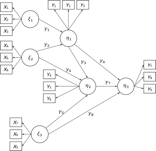
For this study, a more complex model was used, with three exogenous and three endogenous variables. The model is depicted in Figure 7. The data was generated in the same manner as in Study 1. The variances of the exogenous variables ξ1, ξ2, and ξ3 were set at 100, while the residual variances of the endogenous variables η1, η2, and η3were set at 400. Different sample sizes, namely 50, 100, 200, and 300, were used. The coefficient of determination was also varied, namely 0.3, 0.6, 0.7, and 0.9. Combined, this gave 16 conditions.
Analyses
For each condition, 1,000 datasets were generated and then fitted with a correctly specified model, using both SEM and the method of Croon. Then, two criteria were computed, namely the convergence rate and the bias in the regression parameters.
Results
Convergence Rate
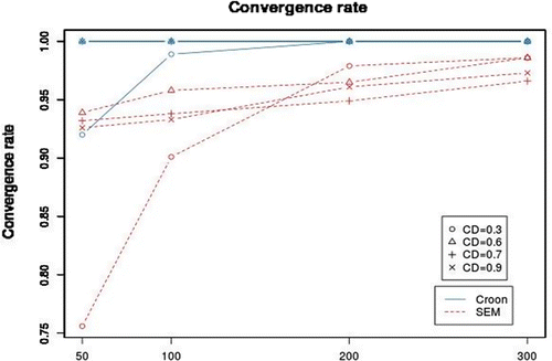
The first criterion is the convergence rate. As can be seen in Figure 8, the proportion is higher for the Croon method than for SEM. The lowest proportion for the method of Croon is 0.92 and there are only two conditions in which the method does not converge every time. These are the conditions with very weak factor loadings (CD = 0.3) and a very small sample size (50 or 100). The lowest proportion for SEM is 0.752. The proportion does increase as the sample size and coefficient of determination increases, but the proportion does not reach 1, even when the sample size is 300. To summarize, the method of Croon converges more often than SEM when the model is complex and the sample size is small.
Bias
The second criterion is the bias in the regression parameters. Since there are three endogenous variables, the regression parameters were divided into three groups, namely γ1−2, γ3−5, and γ6−8. The results are different for the three groups (see Figure 9). For the Croon method, there is almost no bias in all conditions for all three groups. For the SEM method, different patterns can be detected. The first group of parameter estimates, γ1−2, only shows bias when the factor loadings are weak (CD = 0.3) and the sample size is lower than 200. The second group of parameter estimates, γ3−5, shows bias when the factor loadings are weak (CD = 0.3) and the sample size is lower than 300. The third group of parameter estimates, γ6−8, shows bias in almost all conditions. There is only no bias when the factor loadings are strong (CD = 0.9) and the sample size is higher than 50. The difference between the three groups can be explained by looking at the model in Figure 7. The first endogenous variable η1 is only directly influenced by exogenous variables, while the second endogenous variable η2 is also influenced by another endogenous variable (η1) and the third endogenous variable η3 is influenced by both η1 and η2. When combining this information with the results regarding the bias, one could assume that the more complex the model gets, the larger the sample size needs to be to be able to get unbiased parameter estimates.
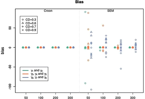
In conclusion, the method of Croon is indeed a better alternative than SEM when the sample size is rather small or the model rather complex. The method of Croon has less problems to converge correctly when the sample size is small and gives less biased estimates of the regression parameter when the model is complex.
Discussion
We compared the method of Croon, a factor score regression method, to SEM using path analysis. The two studies gave us an overall comparison between the performance of SEM and the method of Croon, with regard to the bias and convergence rate. We showed that the method of Croon performs just as well as SEM with regard to bias and convergence rate when path analysis is used. It also handles misspecifications better than SEM and requires a smaller sample size. It can be concluded that the method of Croon can be a suitable alternative for SEM in the setting discussed before.
However, there are some settings in which SEM is still the best alternative. Unless additional restrictions are implemented, factor score regression methods only work when there are at least three items per latent variable. For the moment, the method of Croon also does not work for connected measurement models, such as models with cross-loadings or correlated residual errors. However, we are currently extending the method to be able to handle these kinds of models. We also want to make some extensions to the inference of the model. In future research, we want to use standard errors that are suitable for two-step estimation methods, and we want to develop fit indices, so that the fit of the model can be evaluated, just as in SEM. Finally, we also plan to implement the method in lavaan (Rosseel, 2012).
References
(1937). The statistical conception of mental factors. British Journal of Psychology. General Section, 28, 97–104. doi: 10.1111/j.2044-8295.1937.tb00863.x
(1996). An alternative two stage least squares (2SLS) estimator for latent variable equations. Psychometrika, 61, 109–121. doi: 10.1007/BF02296961
(2002).
Using predicted latent scores in general latent structure models . In G. MarcoulidesI. MoustakiEds., Latent variable and latent structure modeling (pp. 195–223). Mahwah, NJ: Erlbaum.(2016). Hypothesis testing using factor score regression: A comparison of four methods. Educational and Psychological Measurement, 76, 741–770. doi: 10.1177/0013164415607618
(2006). Measurement model quality, sample size, and solution propriety in confirmatory factor models. Multivariate Behavioral Research, 41, 55–64. doi: 10.1207/s15327906mbr4101
(2013).
Bias in factor score regression and a simple solution . In A. R. de LeonK. C. ChoughEds., Analysis of mixed data: Methods & applications (pp. 43–61). Boca Raton, FL: Chapman & Hall. doi: 10.1201/b14571-5(2015). Principles and practice of structural equation modeling (4th ed.). New York, NY: Guilford.
(2011). Two new methods for estimating structural equation models: An illustration and a comparison with two established methods. International Journal of Research in Marketing, 28, 258–268. doi: 10.1016/j.ijresmar.2011.03.006
. (2016). R: A language and environment for statistical computing. Vienna, Austria: R Foundation for Statistical Computing. Retrieved from https://www.r-project.org/
(2012). lavaan: An R package for structural equation modeling. Journal of Statistical Software, 48, 1–36. doi: 10.18637/jss.v048.i02
(1996). A beginner’s guide to structural equation modeling. Mahwah, NJ: Erlbaum.
(2001). Regression among factor scores. Psychometrika, 66, 563–575. doi: 10.1007/BF02296196
(1934). The meaning of i in the estimate of g. British Journal of Psychology, 25, 92–99. doi: 10.1111/j.2044-8295.1934.tb00728.x
(1938). Methods of estimating mental factors. Nature, 141, 246. doi: 10.1038/141246a0
(1935). The vectors of mind. Chicago, IL: University of Chicago Press.
(2003). Indications and limitations of structural equation modeling in complex surveys: Implications for an application in the Medical Expenditure Panel Survey (MEPS). 2003 JSM Proceedings of the American Statistical Associations: Section on survey research methods indications (pp. 4345–4352). San Francisco, CA.


