How to Detect Publication Bias in Psychological Research

Heterogeneity and Bias Detection Methods

Before we turn to our evaluation of the different detection methods, it is worthwhile to briefly discuss a characteristic that most of these methods share: They were designed to address the problem of publication bias in meta-analyses, in which all included primary studies have the same underlying true effect size and differ in their observed effect sizes only because of sampling error (Begg & Mazumdar, 1994; Egger et al., 1997; Ioannidis & Trikalinos, 2007; van Assen et al., 2015).¹ According to two recent surveys (Stanley, Carter, & Doucouliagos, 2018; van Erp et al., 2017), however, between-study heterogeneity is the rule, rather than the exception, in actual psychological meta-analyses. In most meta-analyses the true effect sizes of primary studies appear to vary which may be due to, for example, different operationalizations of the independent variable, different measurements or different participant populations.

For all of the detection methods included here, it can either be deduced from their rationale, or has been shown in previous simulation studies, that their performance will be affected by heterogeneity. This is most easily demonstrated for TIVA: Given that variance in true effect sizes will increase the variance in observed effect sizes, it follows that the conversion of observed p-values into z-scores will, in turn, translate to an increased variance of z-scores. To illustrate this with numbers, we appeal to an example from our study: When we simulated no publication bias and no heterogeneity, we observed an average variance in z-scores that corresponded almost exactly to the expected value of 1 (aggregated across all other conditions of the design, see below). However, when there was a rather moderate degree of heterogeneity (τ = 0.3), the average variance of z-scores was already approximately 2.6. Thus, publication bias is less likely to induce a reduction in variance below the expected value of 1 when there is heterogeneity.

For p-uniform and the regression-based method PET, several simulation studies (e.g., Stanley, 2017; van Aert et al., 2016) demonstrated that, under publication bias and with larger heterogeneity, these tools yield increasingly inflated effect size estimates that more closely resemble the (conventional) meta-analytic effect size estimate. In both cases, this also implies that the signal these methods use to infer the presence of bias (i.e., the inconsistency of the distribution of significant p-values with the meta-analytic effect size estimate for p-uniform, and the relationship between observed effect sizes and their standard errors for PET) is weakened by heterogeneity. Thus, for p-uniform, PET and Begg’s rank correlation (which also relies on the association between observed effect sizes and their standard errors), it has to be expected that these methods lose power under heterogeneity.

Finally, the performance of TES is affected by heterogeneity because its estimation of the power of primary studies relies on the assumption that all of these studies share the same true effect size (Francis, 2013; Ioannidis & Trikalinos, 2007). When there actually is heterogeneity, the resulting estimate of the average power of the primary studies is systematically distorted (Yuan & Maxwell, 2005; this issue will be discussed in more detail below). As a consequence, the expected number of significant results among primary studies will no longer correspond to the observed number of significant results even when there is no bias.

Taken together, these considerations suggest that heterogeneity is an obstacle to the detection of publication bias no matter which of the methods considered here is used. Thus, from a more practical perspective, the choice of a detection method – as well as the interpretation of its results – needs to be informed about its (relative) robustness against heterogeneity. We, therefore, incorporate heterogeneity in the design of our study and aim to provide information pertaining to this problem.

Selection Mechanisms

In the selection condition with no bias, all simulated original studies were published. Hence, this condition served as a control condition which we used to estimate the Type I error rates of the different detection methods. In contrast, in the condition with 100% bias, all simulated nonsignificant results (with α = .05, one-tailed) were excluded from publication. With two further selection mechanisms we implemented a less strict censorship of nonsignificant findings: In the two-step bias condition, “marginally significant” studies with p-values between p = .05 and p = .10 had a 20% chance of being published; studies with p > .10 remained unpublished. In the condition with 90% bias, nonsignificant results were censored with a probability of 90%. In other words, 10% of the simulated primary studies in this condition were published irrespective of their findings.

Finally, in the condition involving not only publication bias but also optional stopping, an initial significance test was performed in all primary studies with a sample size of n = 20 per cell. If the result was nonsignificant, the sample size was increased in either increments of 1 or 5. After each increment, the test for significance was repeated. The procedure was stopped either when a significant result was obtained (in which case the study was published) or when a sample size of n = 40 was reached. Studies that did not find a significant result remained unpublished. By varying the increment in sample size after negative test results, we simulated two different intensities of optional stopping. Both these intensities, however, represent an excessive use of this variant of p-hacking as additional data are collected in all studies that initially find a nonsignificant result.

Mean True Effect Sizes and Degrees of Between-Study Heterogeneity

The four levels of the factor “mean true effect size (δ)” were chosen according to Cohen’s conventions (Cohen, 1988). Heterogeneity was varied in six levels between τ = 0 and τ = 0.5. These levels cover the range of heterogeneity typically observed in psychological meta-analyses (van Erp et al., 2017). In terms of the heterogeneity metric I² (i.e., the ratio of variance in true effect sizes to variance in observed effect sizes), Higgins, Thompson, Deeks, and Altman (2003) proposed to describe values of 0.25, 0.5, and 0.75 as low, medium, and high degrees of heterogeneity. I² depends not only on τ but also on the sample sizes of the primary studies. Within our simulation, random-effects meta-analyses of unbiased study sets yielded average estimates of I² of 0.14, 0.26, 0.42, 0.56, and 0.66 for the τ-values between 0.1 and 0.5, when the mean sample size was n = 25 (no publication bias, aggregated over δ, k and the two conditions with a mean sample size of n = 25). In the three conditions with a mean sample size of n = 50, the respective I² estimates were 0.18, 0.40, 0.59, 0.72, and 0.80.

Sample Sizes of Primary Studies

Sample sizes (n) for experimental and control groups were identical for each individual primary study and drawn from five different uniform distributions that varied in mean and range. Larger mean sample sizes will obviously increase the proportion of significant primary studies in all conditions in which the true effect size δ is larger than zero. Consequently, they will also reduce the proportion of studies that is excluded from publication and may, therefore, affect the performance of bias detection methods. The range of the sample sizes of the studies included in a meta-analysis is of direct importance for Begg’s rank correlation and PET, as these methods assess the covariation between effect sizes and their standard errors. Thus, if there is little variation in sample size (and, therefore, in standard error) the methods are likely to fail. The lower and upper limits of the different uniform distributions in our design roughly correspond to lower and upper quartiles of per-group sample size in four psychological journals as reported by Marszalek, Barber, Kohlhart, and Holmes (2011), for example, Journal of Abnormal Psychology: Q₁ = 10 and Q₃ = 27 in 1977; Journal of Applied Psychology: Q₁ = 21 and Q₃ = 83 in 2006.

Number of Studies per Meta-Analysis

In choosing the levels of this factor, we partly focused on small study sets (k = 5, 7, or 10) as bias detection methods have been applied in rather small samples (e.g., Francis, 2012, 2013), and because we aimed to assess the minimum number of studies necessary for the different methods to achieve acceptable power. According to data collected by van Erp et al. (2017), the median number of studies in psychological meta-analyses is 12. The larger sizes of study sets in our design (k = 30 and 50) roughly correspond to the mean number of studies in psychological meta-analyses and to the 80th percentile.

Procedure

Observations in the control group of each individual study were randomly drawn from a normal distribution with μ = 0 and σ = 1. Observations in the experimental group were also generally generated from a normal distribution with σ = 1. In conditions in which there was no heterogeneity (τ = 0), the mean of this normal distribution was simply equal to the true effect size δ in the given condition. In conditions with heterogeneity, the population mean and, hence, the true effect size for each individual study, was drawn in a preceding step from a normal distribution with μ = δ and σ = τ. For each simulated study, we computed Hedges’ g (as an estimate for the true effect size δ), its variance and standard error (see ESM 1 for details), and determined a one-tailed p-value from an independent samples t-test. Thus, across conditions, studies that were selected for publication based on their p-values generally had a positive effect size.

In each of the 2,640 unique conditions of the complete design, we simulated 1,000 respective meta-analyses. Hence, the maximum standard error (SE) of the proportion of significant results, found by the different detection methods in each of these conditions, is SE = 0.016 (the standard error of an estimated proportion p is given by and will take its maximum value when p = .50).

Bias in Meta-Analytic Effect Size Estimates

Figure 1A shows the mean estimates of meta-analyses for different true effect sizes in all selection conditions when there is no heterogeneity (95% confidence intervals, for all means displayed in Figure 1 have a maximum width of 0.004). In general, when all nonsignificant studies are excluded from publication (i.e., 100% bias), the bias in effect size estimates is fully determined by the average power of the original studies.² Obviously, when there is no true effect (δ = 0), 95% of all studies will be suppressed. Given the sample sizes of original studies in our simulation, the remaining 5% of studies had a weighted mean effect size of  = 0.50, thus giving rise to a very severe overestimation of the true effect size. When the true effect size was δ = 0.2, the average power of simulated original studies was 22% and, consequently, the proportion of censored studies dropped to 78% (see Figure S2 in ESM 1 for power values in all conditions). Meta-analyses of the 22% published studies yielded an average effect size estimate of  = 0.52. Hence, the bias was still large but was also considerably smaller than in the condition with δ = 0. With increasing true effect sizes (and increasing power) the bias decreased further. In the condition with δ = 0.8, it was already almost nil as the average power in this condition exceeded 90% and only relatively few studies were excluded from publication.

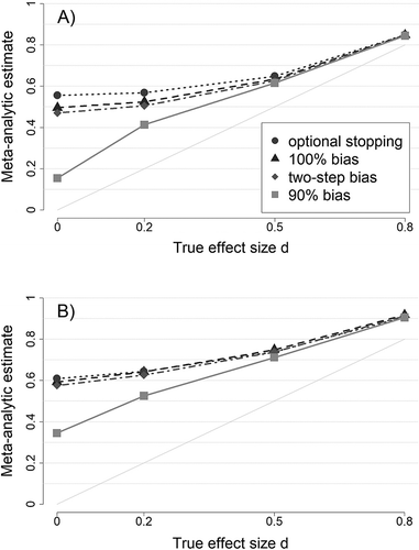
As Figure 1A illustrates, the functional relationship between true effect size and meta-analytic effect size estimates remains unaltered when there is additional optional stopping, or strong but incomplete censoring of marginally significant results. In the latter condition (two-step bias), the bias in effect size estimates was only slightly reduced. This small reduction had to be expected for two reasons: Across all true effect sizes, 92% of published studies in this condition were still significant by the conventional criterion of α = .05 (see Figure S2 in ESM 1; this proportion of significant results among published studies roughly corresponds to estimates of the proportion of significant results in the psychological literature, Fanelli, 2010; Kühberger, Fritz, & Scherndl, 2014). Additionally, marginally significant results are being associated with smaller, but still inflated mean estimates of the true effect sizes.

In contrast, in the condition with additional optional stopping, the bias was slightly amplified. Given the parameter settings of our simulation, optional stopping brought about significant results with smaller sample sizes. The mean sample size of significant studies in the condition with complete publication bias (across all true effect sizes) was n₁ = n₂ = 40.7; in the condition with additional optional stopping, this sample size was n₁ = n₂ = 24.0. Significant results with smaller sample sizes, of course, have to be associated with larger observed effect sizes.

Finally, when 10% of studies were published irrespective of their results, the bias in meta-analytic effect size estimates was greatly reduced. Furthermore, the largest bias no longer occurred at δ = 0 but at δ = 0.2. These findings may appear surprising at first sight, but can be easily deduced: With δ = 0, the proportion of significant results was 5%. Of the remaining 95% of studies, 10% will be published. Thus, even though 90% of studies are produced under publication bias, the proportion of significant results among published studies was only 0.05/(0.05 + 0.95 × 0.10) = 34.5%. The large share of published nonsignificant results reduced the bias drastically ( = 0.15). With δ = 0.2, as reported above, the average power of simulated original studies was 22%. The respective significant studies had a weighted mean effect size of = 0.52 and, thus, still overestimated the true effect size severely. At the same time, the proportion of significant results among published studies increased to 0.22/(0.22 + 0.78 × 0.10) = 73.8%. As a consequence, significant studies had a stronger weight on mean estimates, and the resulting bias was larger than with δ = 0 ( = 0.41; a formal analysis of the relationship between different selection mechanisms and the resulting bias in effect size estimates is given in Ulrich et al., 2018).

Figure 1B shows mean meta-analytic estimates for τ = 0.3, illustrating the effect of heterogeneity on the bias in these estimates. We chose τ = 0.3 for this figure (as well as for Figures 2 and 3) as two recent surveys suggest that the estimated degree of heterogeneity in psychological meta-analyses is typically of about this size (Stanley et al., 2018; van Erp et al., 2017). With growing heterogeneity, the bias in all selection conditions increases. Furthermore, the degree of bias in different selection conditions becomes more similar (see Figure S3 in ESM 1 for mean meta-analytic estimates in all heterogeneity conditions). The general rise in bias is mostly driven by the increased spread of observed effect sizes that is caused by heterogeneity in true effect sizes: Smaller observed effect sizes remain censored due to the significance criterion, whereas larger observed effect sizes are published and, in turn, inflate meta-analytic estimates further.

To summarize, the largest and most relevant biases generally occurred with non-existent or small true effect sizes. With larger effect sizes (and sufficient power), however, the bias tended toward zero. Optional stopping inflated the bias marginally. In contrast, a relatively small proportion of studies that were not subject to censoring were sufficient to decrease the size of bias substantially. Finally, heterogeneity exacerbated biases in effect size estimates resulting from all forms of preferential publication of significant findings. Thus, to avoid seriously wrong conclusions from meta-analytic results, successful bias detection is even more important in the presence of heterogeneity.

Type I Error Rate

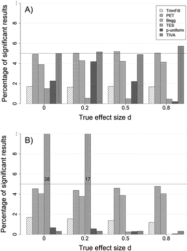
Figure 2 shows the proportion of significant results for all detection methods when there is no publication bias. Under homogeneity (Figure 2A), PET was best at maintaining the nominal α-level, whereas TIVA slightly exceeded it when δ = 0.8 (which is exclusively due to an error rate of 8% with k = 50 studies). The false positive rate of Begg’s rank correlation was at about 4% with all true effect sizes as the method very rarely indicated bias with k = 5 studies (see Figures S4 and S5 in ESM 1). All other methods tended to yield conservative error rates. This tendency was especially pronounced when the number of studies per meta-analysis was small (k ≤ 10) and the true effect size was large (δ ≥ 0.5): Under these circumstances, the Type I error rates of p-uniform, TES, and trim-and-fill often dropped below 1%.

The performance of PET, Begg’s rank correlation and trim-and-fill was hardly affected by heterogeneity (see Figure 2B where τ = 0.3). On the contrary, the false positive rates of TIVA and p-uniform strongly declined with increasing heterogeneity. None of these methods were associated with an appreciably inflated Type I error rate in any combination of true effect size, number of studies and heterogeneity considered here. The striking exception to this rule was TES.

The performance of TES requires some further explanation. When the true mean effect was δ = 0 or δ = 0.2, TES produced an increasingly inflated false positive rate with increasing heterogeneity (see Figure S4 in ESM 1). However, with δ = 0.5 or δ = 0.8, its false positive rate dropped quickly toward zero with increasing heterogeneity. As mentioned before, in TES power is estimated based on the assumption of a fixed-effect model. Thus, when there actually is heterogeneity in true effect sizes, the resulting estimates are systematically distorted. More specifically, when the power estimate of a fixed-effect model is below 50%, the actual power of studies affected by heterogeneity is larger than estimated (Kenny & Judd, 2018; Yuan & Maxwell 2005; this is also discernible by a comparison of the proportion of significant results in the no bias condition under homogeneity and heterogeneity in this simulation, see Figure S2 in ESM 1). This implies that we observed more significant results than expected based on a fixed-effect model power analysis in primary studies with δ = 0 and δ = 0.2. From this difference between the observed and expected number of significant results in primary studies, TES frequently inferred bias even though all studies were properly run and published. In contrast, when the power estimate of a fixed-effect model is above 50%, the actual power of studies affected by heterogeneity is smaller than estimated. Thus, with δ = 0.5 and δ = 0.8, we observed less rejections of the null hypothesis than expected, and consequently, TES very rarely detected an excess of significant findings.³

With δ = 0 and δ = 0.2, severely inflated Type I error rates of TES occurred with as little as 10 studies when τ = 0.3, and with 30 studies when τ = 0.2 (see Figure S4 in ESM 1). As a possible solution to this problem Francis (2013) suggested using a random-effects model to estimate power and to determine the expected number of significant primary studies according to this power estimation. With that said, this procedure is not only analytically much more complex, but we are not aware of any actual application of it. More importantly, power calculation for a random-effects model requires an estimate of τ. These estimates are notoriously imprecise, unless the set of studies is large (Viechtbauer, 2007). Additionally, estimates of τ can and will also be systematically distorted by publication bias (Augusteijn, van Aert, & van Assen, 2019; Jackson, 2007; see also Figure S16 in ESM 1). Given the ubiquity of heterogeneity in psychological meta-analyses (Stanley et al., 2018), we therefore warn against the use of TES in sets of more than 10 studies.

There is one additional, noteworthy restriction to the results depicted in Figure 2: For the evaluation of Begg’s rank correlation and PET, we transformed the effect sizes of the primary studies in a way that stabilized their variance (Hedges, 1981; see ESM 1 for details on this transformation). When these methods were applied to Hedges’ g values directly, they produced inflated false alarm rates for true effect sizes larger than zero (see Figure S6 in ESM 1). This can be explained as follows: Begg’s rank correlation and PET rely on estimates of effect sizes and their standard errors in primary studies. Estimates of the standard error of Hedges’ g depend on the estimate of g itself, in such a way that larger values of g² are associated with larger standard errors (Hedges, 1981). Thus, correlations between observed effect sizes and their standard errors are guaranteed to occur when the true effect size is different from zero. The resulting inflated Type I error rate for Begg’s rank correlation and PET, with g (or r) as effect size measure, has been described before (e.g., Kromrey & Rendina-Gobioff, 2006; Pustejovsky & Rodgers, 2018), but seems to be often times neglected in actual applications of these methods. As a general rule, methods assessing the association between observed effect sizes and their standard errors should only be used after a variance-stabilizing transformation.

Power

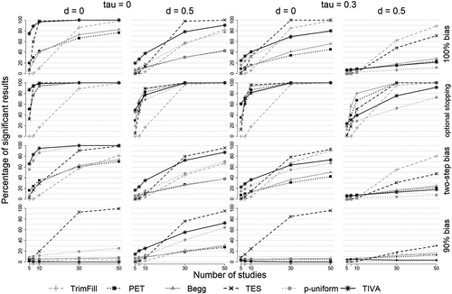
Figure 3 shows the statistical power of each method as a function of selection mechanism, study number, true effect size (only levels δ = 0 and δ = 0.5 shown), and heterogeneity (only levels τ = 0 and τ = 0.3 shown). Power estimates for all simulated effect sizes and degrees of heterogeneity are reported in Figures S7–S12 in ESM 1. In all of these figures, we present power estimates that are averaged across the factor “distribution of sample sizes of primary studies.” Mostly, the effect of this factor on the performance of the different detection methods was small. There were, however, exceptions to this rule that will be described and discussed below.

We organize the description of the statistical power of the detection methods according to selection mechanisms and start out with the 100% bias condition. Results for other selection mechanisms are described subsequently.

When and How Can Publication Biases Be Detected?

Two factors that appear to be of central importance for the detectability of biases are the degree of heterogeneity and the degree of censoring of nonsignificant results. Therefore, we structure the discussion of results on statistical power along two distinctions: one between meta-analyses with homogeneous and heterogeneous effect sizes; one between literatures where nonsignificant results are (almost) fully censored (represented here by the conditions with 100% bias, optional stopping and two-step bias) and literatures where nonsignificant results have an appreciable chance of being published (here, 90% bias).

Let us first consider the combination of homogeneity with complete or severe censorship. Under these circumstances, properly chosen methods often succeeded in detecting the resulting bias in meta-analytic effect size estimates. While several methods performed well, TIVA appeared to be the best available method. In the 100% bias condition, TIVA achieved high statistical power with even as little as 5 studies when the true effect size was δ = 0 and the distortion in effect size estimates was most severe. As had to be expected, the power of all methods increased in larger study sets but declined with larger true effect sizes (and, hence, smaller overestimation). As a consequence, when the true effect was of medium size (δ = 0.5), a reliable detection of biases was only possible in our simulation when at least 30 studies were available. However, TIVA was still the most recommendable option to accomplish this task. When simulated primary studies were additionally affected by optional stopping, the power of all methods increased further. The large gains in power that we observed were certainly due to the specific implementation of optional stopping we realized here. But, as already discussed above, increases in power are likely to also occur when only a portion of researchers is willing to engage in p-hacking or when p-hacking is less intense. TIVA was outperformed by other methods under optional stopping, but this occurred only when the true effect size was large (δ ≥ 0.5). It should be noted that in practice, meta-analysts can know neither the true effect size nor the degree to which available studies are affected by p-hacking. Furthermore, most meta-analysts will likely be most interested in biases that are associated with small or non-existent true effects. Therefore, the observation that other methods performed better when large effects were combined with intense optional stopping gives little reason to prefer these methods. Finally, TIVA’s performance proved relatively robust against the inclusion of some “marginally significant” results in meta-analytic study sets. While its power declined, it nevertheless prevailed over the other methods, and still detected the most severe biases (at δ ≤ 0.2) with high power, when at least 10 studies were available.

The limitations, however, of this positive view, regarding both the detectability of publication biases and TIVA’s performance, become apparent when we follow the distinctions introduced above. Heterogeneity affected the performance of detection methods adversely even when censorship was complete or severe. This occurred even though heterogeneity exacerbated the bias in meta-analytic effect size estimates. For the analysis of real datasets this is of great importance as heterogeneity appears to be the rule rather than the exception in psychological meta-analyses. In a collection of 187 meta-analyses using a standardized mean difference as effect size metric (van Erp et al., 2017), 50% of τ estimates were larger than 0.2, and 30% were larger than 0.3. Under 100% bias and with τ = 0.2, TIVA still achieved acceptable power when the true effect size was small (δ ≤ 0.2) and at least k = 10 studies were available. With τ = 0.3, its power exceeded 50% only when there was no true effect (δ = 0) and the meta-analytic data set comprised 30 or more studies. Furthermore, with a heterogeneity of τ ≥ 0.2, TIVA was almost always outperformed by trim-and-fill in large study sets (k ≥ 30).

This illustrates that there is already no single best method for the detection of publication biases that are caused by a complete suppression of nonsignificant results. Even when no other selection mechanism is considered, an optimal choice of a detection method would require knowledge about the (mean) true effect size and the degree of heterogeneity. Additionally, our results suggest that the detection of biases may quickly become difficult with increasing heterogeneity. Even with moderate degrees of heterogeneity, the power of all methods is rather low in small study sets.

Our second distinction, between an (almost) complete censoring and a censoring that gives nonsignificant results a small chance of being published, is important as it largely separates situations in which bias detection can succeed from situations where it is most likely to fail. In the 90% bias condition, detection methods mostly had small power. When there was a moderate degree of heterogeneity (τ = 0.2), the power of all methods that yielded a proper control of Type I errors was consistently below 30% irrespective of true effect size and number of available studies. Under homogeneity and with δ = 0, TES was the only method that achieved good and even excellent power. Interestingly, TES was clearly the best available option in this specific constellation. Applications of TES, however, will remain doubtful due to the inflated Type I error rate of the method under heterogeneity.

The drop of power observed in the 90% bias condition had to be expected as the resulting bias in meta-analytic effect size estimates was also considerably smaller than in the 100% bias condition. This, however, does not imply that the remaining bias in effect size estimates was irrelevant: In fact, at δ = 0 and τ = 0, the mean effect size estimate was = 0.15. A meta-analytic effect of this size may still give rise to the false impression that there actually is a true effect. Moreover, with some heterogeneity (τ = 0.2 or τ = 0.3), the meta-analytic effect was inflated to a size of about = 0.30. Notably, effect estimates of this size appear to be quite common in psychological meta-analyses (Stanley et al., 2018) and are most likely to lead to the conclusion that a true effect is present. With that said, the power of all detection methods (excluding TES) was reduced to less than 10% even in large study sets. Thus, the combination of a censoring that gives nonsignificant results a small chance of being published with a moderate degree of heterogeneity creates a situation in which the bias in meta-analytic estimates can be both highly relevant, yet also mostly undetected.

Four Recommendations for the Application of Tests for Publication Bias

Given the complexity of the results, one may wonder which practical advice can be given to meta-analysts that aim to assess whether their collection of data is affected by bias. We think that our studies allow for at least four recommendations.

The first of these recommendations is that meta-analysts should strive to avoid heterogeneity before applying methods for the detection of publication bias. Of course, the actual degree of heterogeneity in a collection of studies cannot be known. Furthermore, it can also not be estimated properly in the presence of publication bias. To demonstrate this, Augusteijn et al. (2019) showed analytically that publication bias can have severe and rather complex effects on heterogeneity estimates: Depending on the combination of the actual degree of heterogeneity, true effect size and degree of censorship heterogeneity may either be under- or overestimated. Within the parameter settings of our study, the actual τ was oftentimes underestimated drastically in all four selection conditions realized (see Figure S16 in ESM 1). Hence, even low estimates of τ do not preclude that heterogeneity might actually be large. Consequently, there is no way for meta-analysts to ensure that heterogeneity is small or absent.

However, meta-analysts should be aware that their inclusion criteria for primary studies can partly control the degree of heterogeneity that has to be expected. Primary studies that differ widely in design, procedure, measures, or participant population are likely to be inflicted by more heterogeneity than studies that are methodologically more similar. Our results illustrate that, under publication bias, combining methodologically diverse studies may be a way to both inflate meta-analytic effect size estimates further as well as disguise this bias at the same time. Thus, meta-analysts should decide on plausible moderator variables on theoretical grounds, and apply tests for publication bias to subsets of studies, defined by the different levels of these moderators. The gain in power of the detection methods achieved by reducing heterogeneity will often outweigh the loss induced by the lower number of primary studies available at different moderator levels. Of course, the number of primary studies in a subset should not become too small. That said, there may be solutions to this problem: At least for p-uniform it should be possible to adapt the method in a way that allows to incorporate different meta-analytic effect size estimates per subset, while including all available primary studies in a single test for publication bias.⁵

Our second recommendation concerns the choice of a test for the detection of publication bias. Within our study, TIVA either performed best or at similar levels as any other method as long as censorship was severe and heterogeneity absent or small. With larger degrees of heterogeneity, it was often outperformed by trim-and-fill, especially in large study sets. As will be discussed below, these results may be restricted to the parameter settings simulated here. That said, at least whenever these parameter settings appear plausible, it seems reasonable to apply both these tests. If either of these methods yields a significant result this should be considered a red flag, indicating that meta-analytical results may not be valid. Considering the low Type I error rates of both of these methods in almost all conditions, there is little reason to worry that this multiple testing gives rise to inflated false alarm rates. With regard to trim-and-fill, however, it should be emphasized again that the method may be useful for the detection of biases, but is not recommended for the estimation of true effect sizes when bias is present (Carter et al., 2019; van Aert et al., 2016).

Finally, if a sizeable proportion of the available primary studies is nonsignificant and there is strong reason to assume that these studies are homogeneous (for instance, because the studies can be considered as close replications of each other), it may be advisable to apply TES: TES was the only method providing a reasonable chance to detect bias when censorship was less extreme (in the 90% bias condition). In other words, with the exception of the TES method, biases that may occur even though some studies are published irrespective of their results will mostly remain undetected by all other methods.

The third recommendation pertains to the interpretation of nonsignificant results of bias tests. In view of the rather low power that the detection methods achieve under heterogeneity or with less severe censoring, it is clear that a nonsignificant result of a bias test provides little information, especially when the number of available studies is small. Hence, a nonsignificant result should not be interpreted as evidence for the absence of bias, but simply as the absence of evidence.

Our final recommendation is again justified by the oftentimes low power of detection methods: To raise power, meta-analysts should consider to test for bias at an increased significance level of 10%, at the very least when the test is applied to a small set of studies. Similar suggestions have been made by a number of authors with regard to a variety of detection methods (e.g., Begg & Mazumdar, 1994; Francis, 2013; Ioannidis & Trikalinos, 2007).

Limitations

Even though our simulation investigated a large number of conditions, it still captures only a small sample of the multi-dimensional space representing the ways in which data may be generated, analyzed, and selected for publication. This may pose restrictions to the generalizability of our results to data that were generated or censored under conditions not simulated here.

We used a simple two-group design to simulate data in primary studies and measured the effect size in these primary studies as a standardized mean difference. Obviously, real world research uses a multitude of other (and often more complex) designs and may also employ different effect size measures even in two group comparisons. There are, however, reasons to assume that neither the design of primary studies nor the specific effect size measure is of great importance for our results. Of course, different effect size measures may be converted into each other without affecting effect direction or statistical significance in primary studies. Hence, detection methods that rely on p-values or on power estimates (p-uniform, TIVA, and TES) are by definition independent of specific effect size measures. Stable p-values with different effect metrics also imply that the ratio of effect estimates to their standard errors is stable. This ensures that the results of Begg’s rank correlation and PET remain unaltered across different suitable metrics. Finally, trim-and-fill considers exclusively the rank order of effect sizes – a property that will be invariant across any meaningful transformation of measures.

With regard to design, it is helpful to distinguish between primary studies and meta-analyses summarizing these primary studies. While primary studies may use all kinds of complex multi-factorial designs, most meta-analyses focus on simple contrasts between two conditions. Thus, when extracting information from primary studies, meta-analysts typically aim to compute effect sizes that describe the difference between the two focal conditions, and which are comparable even though the data were collected in different designs. Accordingly, most meta-analyses use standardized mean differences (Cohen’s d or Hedges’ g) or (point-biserial) correlations as effect measures (van Erp et al., 2017; Fanelli, Costas, & Ioannidis, 2017). As such, in principle our results should be applicable to all meta-analyses proceeding in this way.

There are, however, constraints on the generalizability of our findings that we deem as more relevant: A recurring theme of our summary of the results has been that a performance assessment of detection methods does not generalize across different simulated selection mechanisms, true effect sizes or degrees of heterogeneity. The results also demonstrate that the performance of the methods depends on the power of primary studies – and, therefore, on their sample sizes. With regard to true effect sizes and degrees of heterogeneity, the parameter settings simulated here may cover a broad range of values that appear plausible in psychology. This is, however, certainly not true for selection mechanisms and sample sizes.

Sample sizes in a given area of research may easily differ, in their mean or variance, from what we simulated here. Furthermore, the distribution of sample sizes of psychological studies appears to be right-skewed (Marszalek et al., 2011). Hence, actual meta-analyses may easily include one or a few studies with unusually large sample sizes. Larger mean sample sizes will generally decrease the detectability of biases which may, additionally, occur at different rates for different detection methods, depending on a variety of other factors (e.g., heterogeneity). We already touched upon the relevance of variance in sample sizes when we presented the results for Begg’s rank correlation and PET. These methods attain higher statistical power when the variation in sample sizes increases (which may, of course, also be caused by a few outliers). In contrast, TIVA’s power is likely to be reduced by larger variation in sample sizes as this variation will also increase the variance of converted z-scores. The different levels of variation realized here had surprisingly little impact on TIVA’s power. Still, it has to be expected that larger variation would diminish TIVA’s performance and may cause Begg’s rank correlation and PET to be the more sensitive methods.

The mechanisms by which real world studies are selected for publication may differ from the selection mechanisms that we simulated in a number of ways: Censoring of nonsignificant results may be less severe, the functional relationship between p-values and publication probabilities may take a different form, and publication probabilities may be affected by factors other than p-values. It is possible that even small deviations from the selection mechanisms simulated here can alter the performance of detection methods severely. For example, the comparatively good performance of trim-and-fill that we observed in many conditions with large study sets may very well be limited to the strict one-sided censoring of studies simulated here. Specifically, it is known that trim-and-fill fails to detect bias when a single unusually small or negative effect size is included in the meta-analytic data set (Duval & Tweedie, 2000; Duval, 2005). In real datasets, such an outlier in the distribution of effect sizes may, of course, occur due to reasons that are totally unrelated to the p-value of the respective study. More generally, many of our results may not generalize to selection mechanisms that assign a non-zero probability of publication to negative significant results. This is easily illustrated with PET. When negative significant results are published with a small probability, they will appear as outliers in a funnel plot. Obviously, these outliers will affect the regression slope that PET uses to diagnose bias.

Overall, the ways in which characteristics of primary studies and features of the publication process impact the performance of detection methods are likely to be even more complex than suggested by our results. It should be noted that this also qualifies our recommendation for TIVA and trim-and-fill: These methods can only be expected to show a comparatively good performance in situations in which it seems plausible that the conditions simulated here in fact apply.

A final limitation of our study concerns the detection methods that we evaluated. The performance of most of these methods deteriorated under heterogeneity. This suggests that methods might fare better if they explicitly take into account that primary studies may have heterogeneous effect sizes. Indeed, there is a class of methods that do exactly this: Selection model approaches (e.g., Hedges, 1984; Iyengar & Greenhouse, 1988; Hedges & Vevea, 1996; Copas & Shi, 2000) combine a model of the data generation process with a model of the selection process to mitigate bias. Maximum likelihood techniques are used to estimate the parameters of these models. For instance, the parameters of the three-parameter selection model (Iyengar & Greenhouse, 1988) are δ, τ, and the probability p that a nonsignificant study gets published. Thus, the method provides corrected estimates of the true effect size and the degree of heterogeneity, and allows for a statistical test of the hypothesis that bias is present as based on the parameter p. We did not include selection model approaches here because one of our goals was to assess the minimum number of studies necessary to detect bias. This led us to focus on meta-analyses that include only a small number of primary studies (k ≤ 10). In such small study sets, selection model approaches can be expected to have severe convergence problems (Field & Gillett, 2010) and will often not yield any results at all. Thus, it is unlikely that they outperform the methods considered here when only a small number of studies are available. In larger study sets, however, they are certainly a viable option. Notably, a recent simulation study (Pustejovsky & Rodgers, 2018) found that the three-parameter selection model performed comparatively well and may be the preferable choice in sets including 20 or more studies.

How to Interpret a Significant Result of a Bias Test

We already pointed out that nonsignificant results of bias tests will typically provide little information. However, the interpretation of significant results of bias tests also entails some problems that should not be neglected.

Under severe publication bias, all of the detection methods considered here attained the highest statistical power when there was no true effect and the resulting distortion in the meta-analytic effect size estimate was particularly pronounced. However, biases may and will also be detected when there is a true effect and the distortion in meta-analytic estimates is reduced. In the 90% bias condition, TIVA and p-uniform detected even more biases with small or moderate true effect sizes than with δ = 0. Obviously, then, a significant bias test does not allow for the conclusion that there is no true effect. Furthermore, a significant result that occurs with a medium effect size of δ = 0.5 will (mostly) correctly indicate that the meta-analytic effect size estimate is not valid. At the same time, the distortion in this estimate will often be relatively small and may be of little relevance for any substantive interpretation. Thus, it remains unclear what should be concluded from a significant bias test with regard to the effect under investigation. For this reason, methods that are not only capable to detect but also correct biases in meta-analytic effect size estimates are desirable. The results of simulation studies on such corrected estimates, however, are not very encouraging (Carter et al., 2019; McShane et al., 2016). Thus, there is good reason to assume that methods for the correction of bias, when applied to real world meta-analyses, will rarely converge into an estimate that appears trustworthy and reliable. The only justifiable conclusion from a significant result of a publication bias test will, therefore, often be that the meta-analytic effect size estimate is not valid and does not allow for any substantive claim about the effect under investigation.

The second caveat for the interpretation of a significant result of a bias test stems from the fact that none of the detection methods actually tests “directly” for publication bias. All of the detection methods search for some signal in the available data that occurs when bias is present (e.g., an association between effect sizes and their standard errors, or an irregularity in the distribution of p-values). Therefore, a significant result can only be interpreted as an indication of bias to the degree to which alternative explanations for the occurrence of the respective signals can be excluded. In principle, there are always alternative explanations to publication bias, no matter which method was used to detect such bias. Within our simulation, this is apparent for TES. Here, the alternative explanation for a significant result is simply heterogeneity. In real datasets, however, there may also be benign causes for an association between observed effect sizes and their standard errors and, thus, for a significant result of Begg’s rank correlation or PET. Such an association may occur, for instance, when true effect sizes vary systematically and researchers successfully adapt their sample sizes to these true effect sizes (Sterne et al., 2000). Similarly, it has been shown that no specific distribution of p-values implies a specific selection process (Ulrich & Miller, 2015). Thus, while significant results for p-uniform and TIVA do in fact suggest selective reporting (i.e., that not all results of primary studies are included in the meta-analysis), they do not necessarily imply that the selection process had a preference for significant or small p-values in primary studies. In other words, significant results for these detection methods are not by default a function of excluding nonsignificant primary studies; moreover, they may also not indicate an overestimation of true effect sizes (Erdfelder & Heck, 2019). Thus, it is important to emphasize that, in general, no detection method can yield “proof” of bias. Therefore, a careful interpretation of the results of these methods requires a consideration of alternative explanations.

Conclusion

To conclude, we may ask what can be achieved by detection methods. As we have seen, these methods can uncover biases with high statistical power when censoring of nonsignificant results is very severe and true effect sizes are homogeneous. Properly chosen methods may even accomplish this in small study sets. This provides a sufficient reason to use such methods at all. For instance, TIVA or p-uniform may be used to identify multi-study papers that test a hypothesis in several experiments and present a doubtful conclusion. However, across all data generation and selection processes that appear to be realistic in the psychological literature, there is neither a single “best” detection method nor will any method be able to separate biased data collections from unbiased data collections reliably. Under many scenarios, relevant biases in meta-analytic effect size estimates are likely to remain undetected. On the other hand, biases that are detected may be small and of little relevance for any substantive interpretation. This implies that not only detection methods but also the meta-analyses themselves, will not yield any definite conclusions as long as publication biases and questionable research practices have to be expected in the psychological literature. Thus, our results may be understood as a plea for open science practices: If there is doubt on the trustworthiness of the available evidence on a specific research question, then any attempt to resolve this will ultimately have to rely on large-scale, preregistered replications. In the future, we should produce and publish evidence that is of better quality in the first place. Preregistrations and openly available data should become standard for all primary studies. In essence, publication decisions should no longer depend on statistical results but on theoretical and methodological soundness.

References

. (2010).
Meta-analysis reporting standards (MARS) . In American Psychological AssociationEd., Publication Manual of the American Psychological Association (pp. 245–254). Washington, DC: Author.(2019). The effect of publication bias on the Q test and assessment of heterogeneity. Psychological Methods, 24, 116–134. https://doi.org/10.1037/met0000197
(1994). Operating characteristics of a rank correlation test for publication bias. Biometrics, 50, 1088–1101. https://doi.org/10.2307/2533446
(2016). Problems in using p-curve analysis and text-mining to detect rate of p-hacking and evidential value. PeerJ, 4, e1715. https://doi.org/10.7717/peerj.1715
(2017). D-cycloserine augmentation of behavior therapy for anxiety and obsessive-compulsive disorders: A meta-Analysis. PLoS One, 12, e0173660. https://doi.org/10.1371/journal.pone.0173660
(2019). Correcting for bias in psychology: A comparison of meta-analytic methods. Advances in Methods and Practice in Psychological Science, 2, 115–144. https://doi.org/10.1177/2515245919847196
(1988). Statistical power analysis for the behavioral sciences (2nd ed.). Hillsdale, NJ: Erlbaum.
(2000). Meta-analysis, funnel plots and sensitivity analysis. Biostatistics, 1, 247–262. https://doi.org/10.1093/biostatistics/1.3.247
(1986). Meta-analysis in clinical trials. Controlled Clinical Trials, 7, 177–188. https://doi.org/10.1016/0197-2456(86)90046-2
(2005).
The trim and fill method . In H. R. RothsteinA. J. SuttonM. BorensteinEds., Publication bias in meta-analysis: Prevention, assessment and adjustments (pp. 127–144). Chichester, UK: Wiley.(2000). Trim and fill: A simple funnel-plot-based method of testing and adjusting for publication bias in meta-analysis. Biometrics, 56, 455–463. https://doi.org/10.1111/j.0006-341X.2000.00455.x
(1997). Bias in meta‐analysis detected by a simple graphical test. British Medical Journal, 315, 629–634. https://doi.org/10.1136/bmj.315.7109.629
(2019). Detecting evidential value and p-hacking with the p-curve tool: A word of caution. Zeitschrift für Psychologie, 227, 249–260. https://doi.org/10.1027/2151-2604/a000383
(2010). “Positive” results increase down the hierarchy of the sciences. PLoS One, 5, e10068. https://doi.org/10.1371/journal.pone.0010068
(2017). Meta-assessment of bias in science. Proceedings of the National Academy of Science of the United States of America, 114, 3714–3719. https://doi.org/10.1073/pnas.1618569114
(2010). How to do meta-analysis. British Journal of Mathematical and Statistical Psychology, 63, 665–694. https://doi.org/10.1348/000711010X502733
(2012). The same old new look: Publication bias in a study of wishful seeing. i-Perception, 3, 176–178. https://doi.org/10.1068/i0519ic
(2013). Replication, statistical consistency, and publication bias. Journal of Mathematical Psychology, 57, 153–169. https://doi.org/10.1016/j.jmp.2013.02.003
(1981). Distribution theory for Glass’s estimator of effect size and related estimators. Journal of Educational Statistics, 6, 107–128. https://doi.org/10.3102/10769986006002107
(1984). Estimation of effect size under nonrandom sampling: The effects of censoring studies yielding statistically insignificant mean differences. Journal of Educational and Behavioral Statistics, 9, 61–85. https://doi.org/10.3102/10769986009001061
(1996). Estimating effect size under publication bias: Small sample properties and robustness of a random effects selection model. Journal of Educational and Behavioral Statistics, 21, 299–332. https://doi.org/10.2307/1165338
(2003). Measuring inconsistency in meta‐analyses. British Medical Journal, 327, 557–560. https://doi.org/10.1136/bmj.327.7414.557
(2007). An exploratory test for an excess of significant findings. Clinical Trials: Journal of the Society for Clinical Trials, 4, 245–253. https://doi.org/10.1177/1740774507079441
(1988). Selection models and the file drawer problem. Statistical Science, 3, 109–117. https://doi.org/10.1214/ss/1177013012
(2007). Assessing the implications of publication bias for two popular estimates of between-study variance in meta-analysis. Biometrics, 63, 187–193. https://doi.org/10.1111/j.1541-0420.2006.00663.x
(2018, September 15). The unappreciated heterogeneity of effect sizes: Implications for power, precision, planning of research, and replication. Retrieved from http://davidakenny.net/recp.htm
(2006). On knowing what we do not know. An empirical comparison of methods to detect publication bias in meta-analysis. Educational and Psychological Measurement, 66, 357–373. https://doi.org/10.1177/0013164405278585
(2014). Publication bias in psychology: A diagnosis based on the correlation between effect size and sample size. PLoS One, 9, e105825. https://doi.org/10.1371/journal.pone.0105825
(2011). Sample size in psychological research over the past 30 years. Perceptual and Motor Skills, 112, 331–348. https://doi.org/10.2466/03.11.PMS.112.2.331-348
(2001). A comparison of methods to detect publication bias in meta-analysis. Statistics in Medicine, 20, 641–654. https://doi.org/10.1002/sim.698
(2016). Adjusting for publication bias in meta-analysis: An evaluation of selection methods and some cautionary notes. Perspectives on Psychological Science, 11, 730–749. https://doi.org/10.1177/1745691616662243
(2013). The consistency test does not – and cannot – deliver what is advertised: A comment on Francis (2013). Journal of Mathematical Psychology, 57, 180–183. https://doi.org/10.1016/j.jmp.2013.03.004
. (2015). Estimating the reproducibility of psychological science. Science, 349(6251). https://doi.org/10.1126/science.aac4716
(2018). Testing for funnel plot asymmetry of standardized mean differences. Research Synthesis Methods, 10, 57–71. https://doi.org/10.1002/jrsm.1332
(2011). Detecting and adjusting for small-study effects in meta-analysis. Biometrical Journal, 53, 351–368. https://doi.org/10.1002/bimj.201000151
(2014, December 30). The test of insufficient variance (TIVA): A new tool for the detection of questionable research practices [Blog Post]. Retrieved from http://replicationindex.wordpress.com/2014/12/30/the-test-of-insufficient-variance-tiva-a-new-tool-for-the-detection-of-questionable-research-practices/
(2011). False-positive psychology: Undisclosed flexibility in data collection and analysis allows presenting anything as significant. Psychological Science, 22, 1359–1366. https://doi.org/10.1177/0956797611417632
(2013). It really just does not follow, comments on Francis (2013). Journal of Mathematical Psychology, 57, 174–176. https://doi.org/10.1016/j.jmp.2013.03.006
(2014). P-curve and effect size: Correcting for publication bias using only significant results. Perspectives on Psychological Science, 9, 666–681. https://doi.org/10.1177/1745691614553988
(2017). Limitations of PET-PEESE and other meta-analysis methods. Social Psychological and Personality Science, 8, 581–591. https://doi.org/10.1177/1948550617693062
(2018). What meta-analyses reveal about the replicability of psychological research. Psychological Bulletin, 144, 1325–1346. https://doi.org/10.1037/bul0000169
(2014). Meta-regression approximations to reduce publication selection bias. Research Synthesis Methods, 5, 60–78. https://doi.org/10.1002/jrsm.1095
(2000). Publication and related bias in meta-analysis: Power of statistical tests and prevalence in the literature. Journal of Clinical Epidemiology, 53, 1119–1129. https://doi.org/10.1016/S0895-4356(00)00242-0
(2003). Adjusting for publication bias in the presence of heterogeneity. Statistics in Medicine, 22, 2113–2126. https://doi.org/10.1002/sim.1461
(2015). P-hacking by post hoc selection with multiple opportunities: Detectability by skewness test? Comment on Simonsohn, Nelson and Simmons (2014). Journal of Experimental Psychology: General, 144, 1137–1145. https://doi.org/10.1037/xge0000086
(2018). Effect size estimation from t statistics in the presence of publication bias: A brief review of existing approaches with some extensions. Zeitschrift für Psychologie, 226, 56–80. https://doi.org/10.1027/2151-2604/a000319
(2016). Conducting meta-analyses based on p values: Reservations and recommendations for applying p-uniform and p-curve. Perspectives on Psychological Science, 11, 713–729. https://doi.org/10.1177/1745691616650874
(2019). Publication bias examined in meta-analyses from psychology and medicine: A meta-meta-analysis. PLoS One, 14, e0215052. https://doi.org/10.1371/journal.pone.0215052
(2015). Meta-analysis using effect size distributions of only statistically significant studies. Psychological Methods, 20, 293. https://doi.org/10.1037/met0000025
(2017). Estimates of between-study heterogeneity for 705 meta-analyses reported in Psychological Bulletin from 1990–2013. Journal of Open Psychology Data, 5, 4. https://doi.org/10.5334/jopd.33
(2007). Confidence intervals for the amount of heterogeneity in meta-analysis. Statistics in Medicine, 26, 37–52. https://doi.org/10.1002/sim.2514
(2016). Registered replication report: Strack, Martin, and Stepper (1988). Perspectives on Psychological Science, 11, 917–928. https://doi.org/10.1177/1745691616674458
(2018). Null effects of perceptual disfluency on learning outcomes in a text-based educational Context: A meta-analysis. Educational Psychology Review, 30, 745–771. https://doi.org/10.1007/s10648-018-9442-x
(2005). On the post hoc power in testing mean differences. Journal of Educational and Behavioral Statistics, 30, 141–167. https://doi.org/10.3102/10769986030002141